Geophysics Weekly – 28 August 2026
S. G.
- / -
Physics and numerics of variably saturated porous media
Modelling continental-scale groundwater flow
Sia Ghelichkhan, Liam Morrow, Stephan Kramer, and the whole team
Geophysics Weekly, 28 August 2026
What I actually want to say
- Physics of groundwater flow can be genuinely tricky.
Ultimate Goal: digital twin for water resources (akin to weather forecasting).
We have done the forward modelling part.
Everything else today serves the above statements.
A bit of global hydrology
for geophysicists
The hydrological cycle = conservation of mass
- Movement of water between atmosphere, ocean, ice, surface and subsurface as gas, liquid and solid.
A large part of the action happens underground, out of sight.
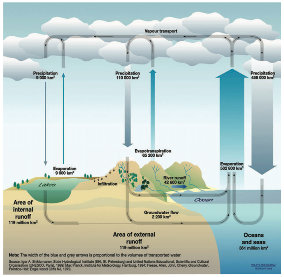
Hydrology is the science of bookkeeping: whatever enters a volume, minus whatever leaves.
Hydrology: the biggest misnomer ever
| Storage | Volume (×10³ km³) | % of total |
|---|---|---|
| Oceans/seas | 1,338,000 | 96.54 |
| Ice caps/glaciers | 24,064 | 1.74 |
| Groundwater | 23,400 | 1.69 |
| Permafrost | 300 | 0.022 |
| Lakes | 176 | 0.013 |
| Soil | 16.5 | 0.001 |
| Atmosphere | 12.9 | 0.0009 |
| Marsh/wetlands | 11.5 | 0.0008 |
| Rivers | 2.12 | 0.00015 |
| Biota | 1.12 | 0.00008 |
| Total | 1,385,984 | 100.00 |
Discount the ocean and the ice.
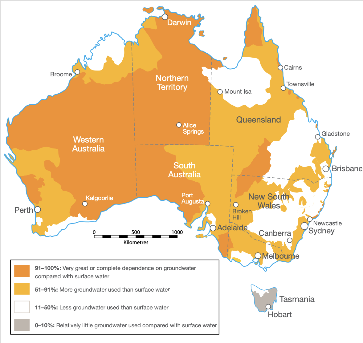
groundwater is ~99% of the unfrozen fresh water on the planet.
- It supplies about half of domestic water use worldwide.
- It supplies over 40% of the water used for irrigation.
The continental water balance, and who owns each term
Given to us
Comes from the climate system. We take it as forcing. We are essentially powerless over it.
Mostly forced
Set by temperature, water availability and aerodynamics (wind). Largely dictated to us.
Ours to model
This is the subsurface. This is where the physics is, and where we come in.
The balance funnels us straight to the term we can actually compute: the water below the surface.
Model and forecast water resources
Two stores, very different behaviour:
- Surface water - rivers, dams, lakes. Highly visible, but set largely by topography and by this year’s rainfall. It rises and falls fast.
- Groundwater - the slow, buffered store. It integrates decades of recharge and keeps rivers alive through drought (baseflow).
This is the case for focusing on groundwater: it is not only the biggest accessible fresh-water store, it is the most reliable one. The buffer that carries a catchment through a dry decade.
Surface and subsurface flow are inseparable. 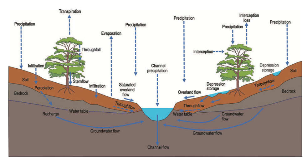
Forecasting (modelling) Groundwater
Groundwater flow cannot be observed directly.
- The subsurface is sampled only at scattered boreholes.
- Conductivity and storativity are known, if at all, at a handful of points.
- Through surrogate methods, variations can be observed. satellite geodesy, seismology.
- You cannot interpolate/extrapolate between boreholes: the water between them moves by physical law, not by an assumption of smoothness.
Recovering the flow needs a model. That splits the problem in two:
A forecast needs two components. And an efficient inverse needs the forward solver plus its sensitivities. So the forward solver is the foundation – build that first.
Forward problem
Physics + material properties + forcing
Inverse problem
Sparse observations
The forward physics
From Darcy to Richards
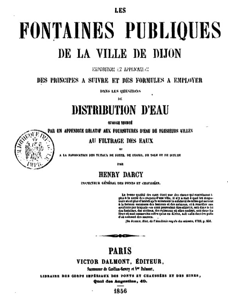
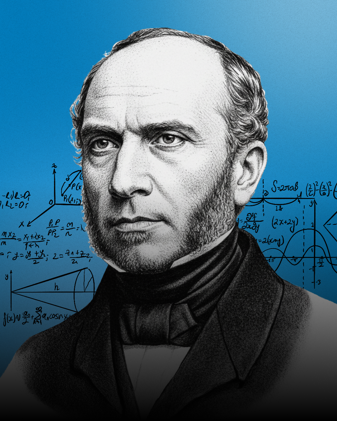
Father of Quantitative Hydrogeology
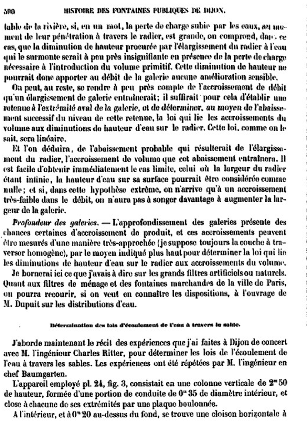
AI Translation: ”… the experiments I carried out at Dijon together with the engineer M. Charles Ritter, to determine the laws of the flow of water through sands. The experiments were repeated by the chief engineer M. Baumgarten.”
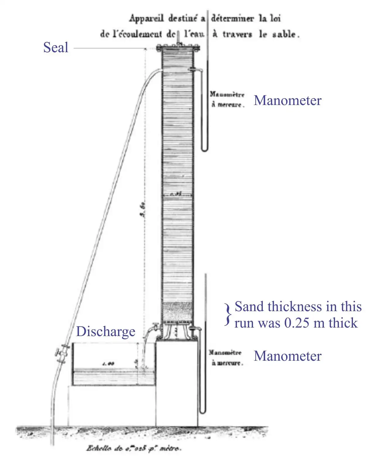
”… there is a linear relationship between the head and the volume you are getting out of the filter”
Darcy principles
Darcy (1856), studying sand columns for Dijon’s water supply, gave the momentum balance for slow flow through a porous medium:
Combine it with conservation of mass and you get the classical groundwater-flow equation:
In the saturated zone
But the subsurface at large is not fully saturated.
Notation
H = h + z : total headh : pressure head (h = p/\rho g )z : elevation head (gravity)
Saturated:
Subsurface is not only the saturated zone
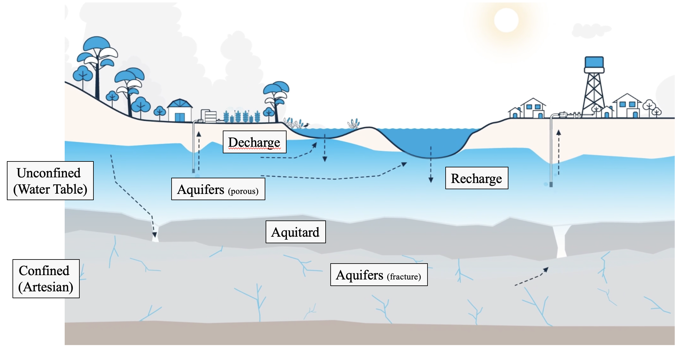
So much interesting stuff happens in the vadose zone
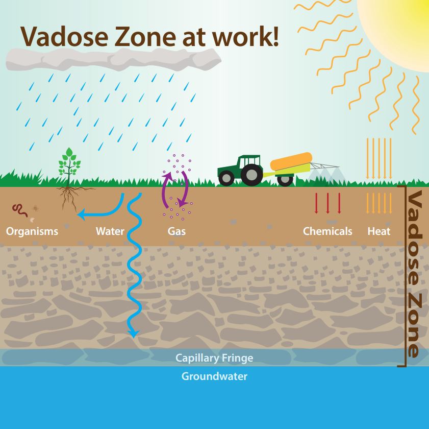
- Agriculture: soil moisture sets crop yield and irrigation demand.
- Recharge: it decides how much rain actually reaches the aquifer.
- Bushfire: dry soil means dry fuel; a leading indicator of fire danger.
- Contamination: nitrate, pesticides, PFAS, spills all enter groundwater through it.
and here we are …
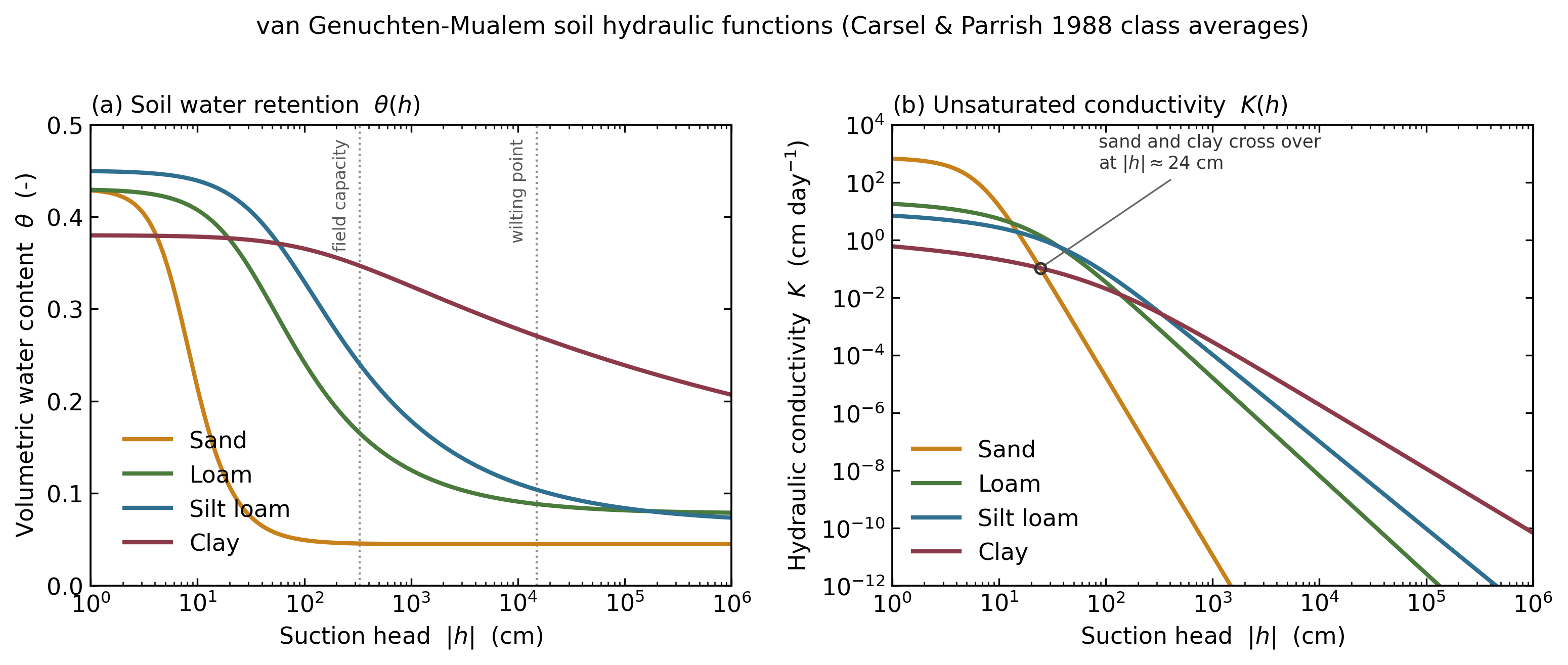
The soil turns the constants into curves: moisture
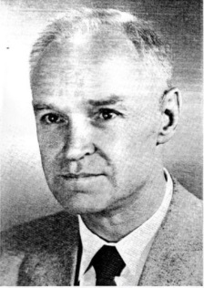
Lorenzo Richards
The vadose zone: constants become functions
Above the water table lies the unsaturated (vadose) zone. Pores hold both air and water, and the water is held under negative (capillary) pressure.
Darcy’s law still holds. What changes is that the coefficients now depend on the state:
- Conductivity collapses as the soil dries:
K(h) = K_s \, k_r(h) , falling many orders of magnitude. - Storage depends on the moisture the pressure sets up.
Both the stored water and its ability to move depend on the pressure head that the flow itself produces. The balance becomes nonlinear - and the linear, MODFLOW-type description no longer holds.
Conductivity and moisture as functions of the head.
Richards’ equation
Darcy in the unsaturated zone,
\theta(h) : volumetric moisture content\theta = \theta(h) K(h) : hydraulic conductivity;K = K_s \, k_r(h) z : elevation head – the gravity term that drives percolations : sources and sinks (recharge, extraction)
Degenerate at both ends:
- Dry soil,
K \to 0 : the flux collapses, infiltration advances as a sharp front. - Fully saturated,
\theta constant: the time derivative vanishes, the equation turns elliptic.
This shifting character is what makes it notoriously hard to solve.
Reliability
Are the solutions accurate?
Scalability
Can we solve a very big system? (high # of DoF)
Flexibility
Terrain-following meshes and a choice of discretisation?
Connection to data
Real elevation, stratigraphy and borehole observations?
Inversion
Can we do gradient-based (adjoint) optimisation?
Our solver: Richards’ equation inside G-ADOPT
Built in G-ADOPT (the Geoscientific ADjoint Optimisation Platform) on Firedrake, PETSc and pyadjoint - the same stack we use for mantle and lithosphere dynamics, now pointed at the near surface.
- Discontinuous Galerkin discretisation: locally mass-conservative, tolerant of sharp fronts and material jumps.
- Newton iteration on an exact, symbolically derived Jacobian.
- Implicit Runge-Kutta time stepping (Irksome); Backward Euler here.
- Anisotropy-aware multigrid preconditioning that coarsens to match the thin-sheet aspect ratio.
- Terrain-following mesh assembled from a national elevation model and borehole stratigraphy.

Verification of the solvers
Or the part I convince you it does!
Verification: accuracy and strict mass conservation
We check the solver against a suite of benchmarks:
- Tracy (2002) - an analytic solution. The strictest test: no reference-solution ambiguity.
- Vauclin (1979) - a measured water-table recharge experiment, compared against four independent codes.
- Mass conservation - local and global mass balance held to round-off.
- A heterogeneous 3D case (Cockett 2018) - a realistic test before we extend to continental scale.
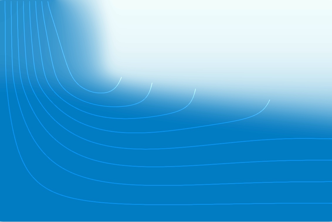
Vauclin: localised recharge builds a wetting front and a groundwater mound – unsaturated percolation and saturated flow in one equation.
Tracy (2006): an exact solution to check against
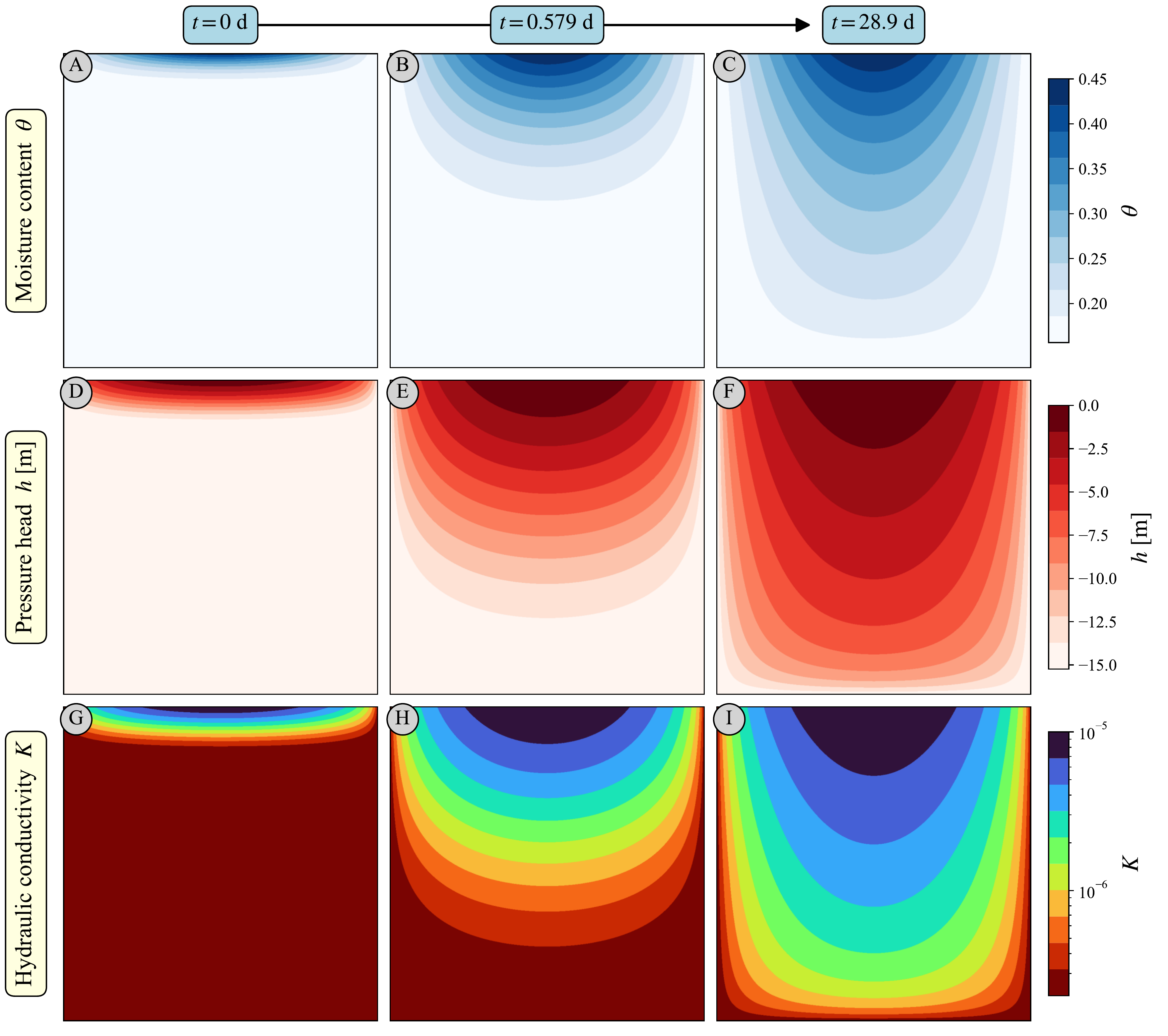
Head evolving to steady state at
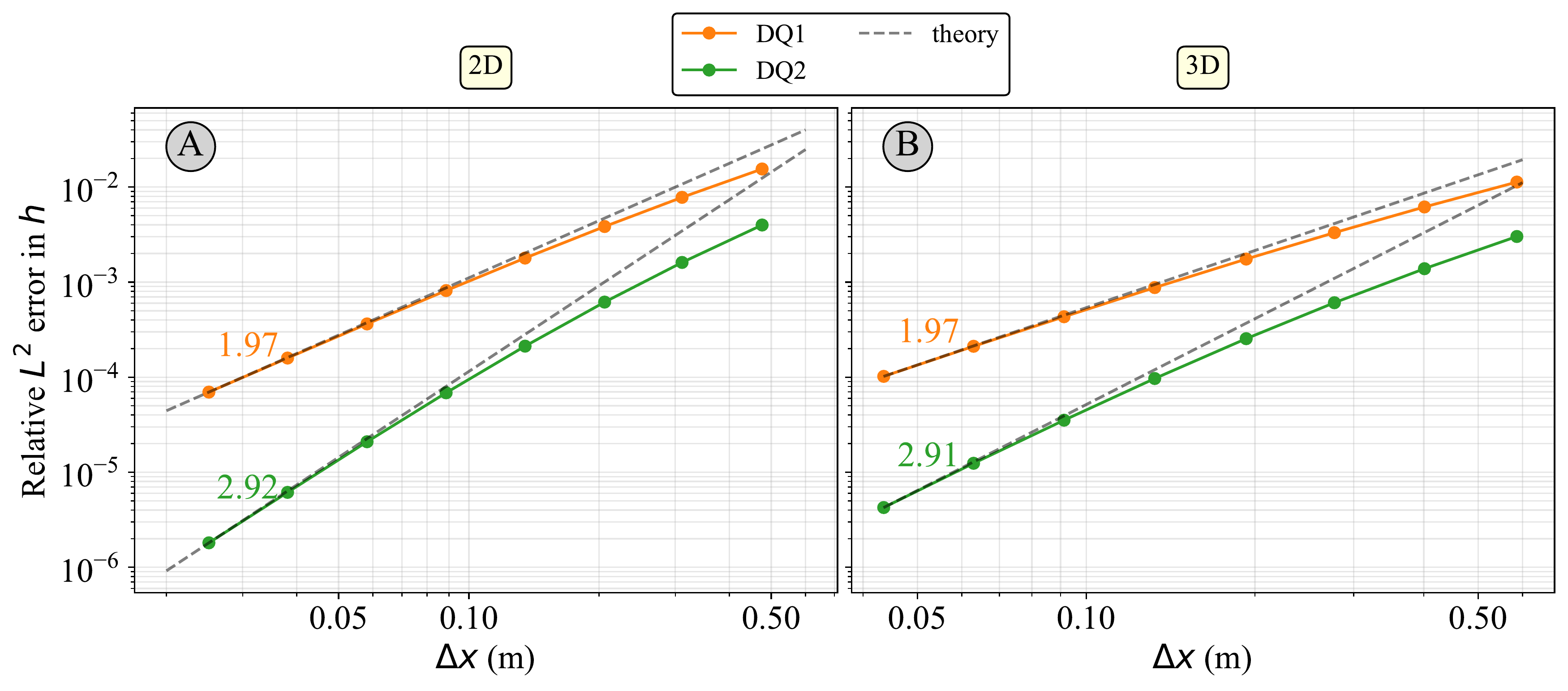
Why Tracy? An exact solution to Richards’ equation – so we measure the true error, not code-versus-code.
- Exponential soil,
\theta,\,K \propto e^{\alpha h} , linearises the equation and admits an analytic solution. - Square domain,
15.24 \times 15.24 m. A sinusoidal head on the top boundary drives infiltration into initially dry soil. \alpha = 0.25 /m,\theta_r = 0.15 ,\theta_s = 0.45 ,K_s = 10^{-5} m/s.- Driven to steady state with Backward Euler.
Spatial error converges at the optimal rate
Testing the numerical solutions versus theory
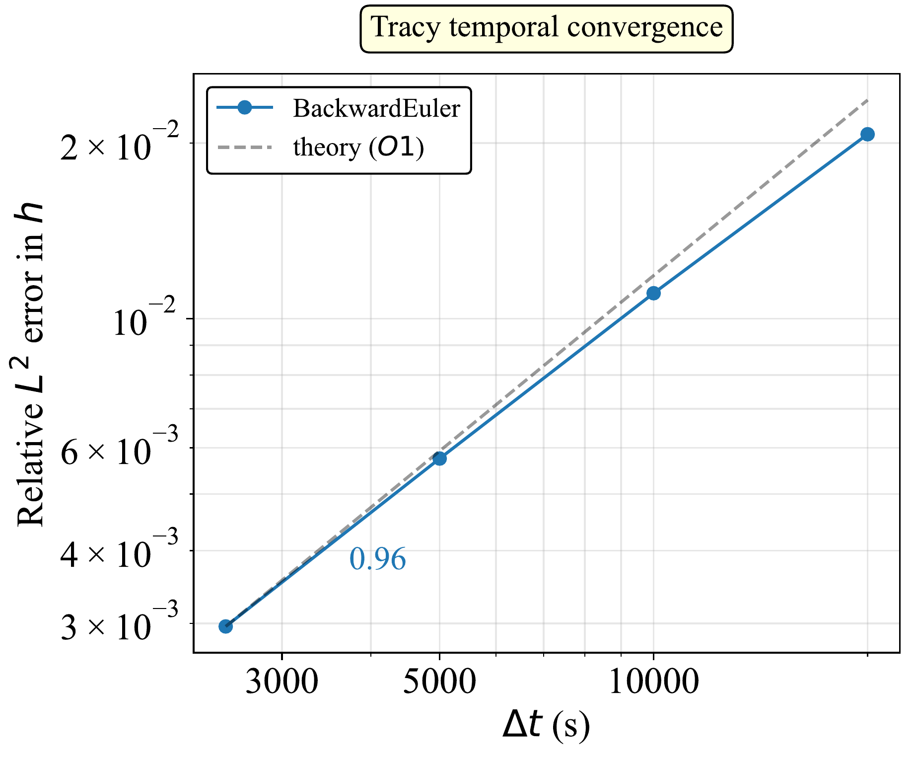
Backward Euler: first-order accurate in time,
Testing mass conservation
Most fundamental constraint in hydrology: No drop left behind
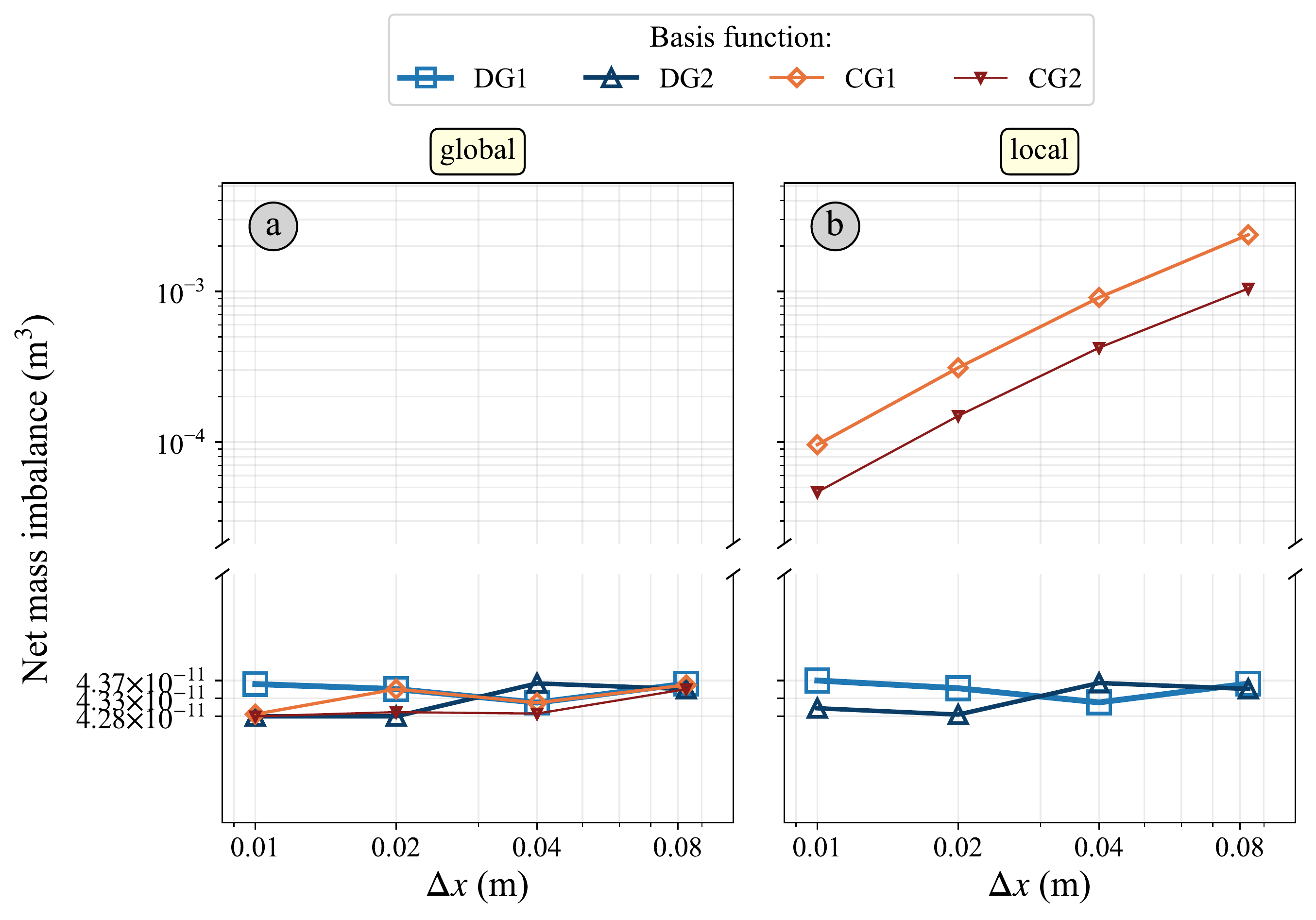
Discontinuous Galerkin conserves water locally, cell by cell, to the tolerance of the nonlinear solve.
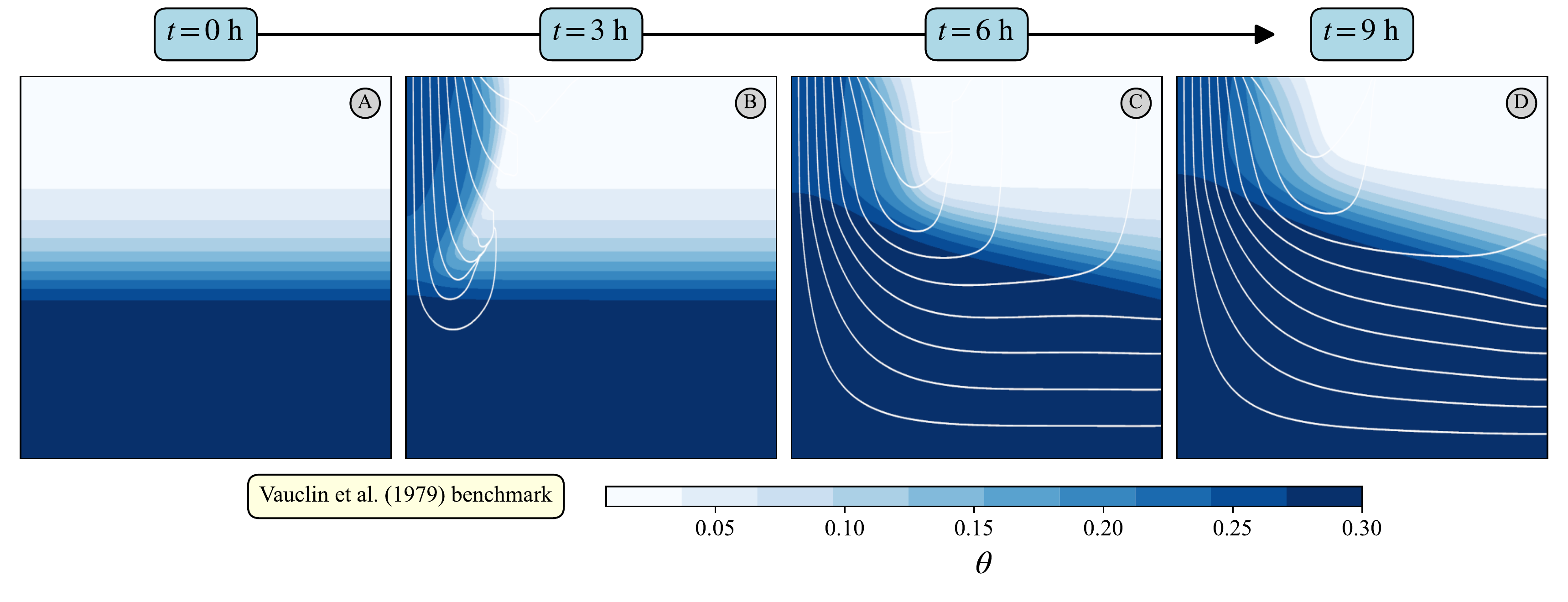
Vauclin (1979): moisture content at
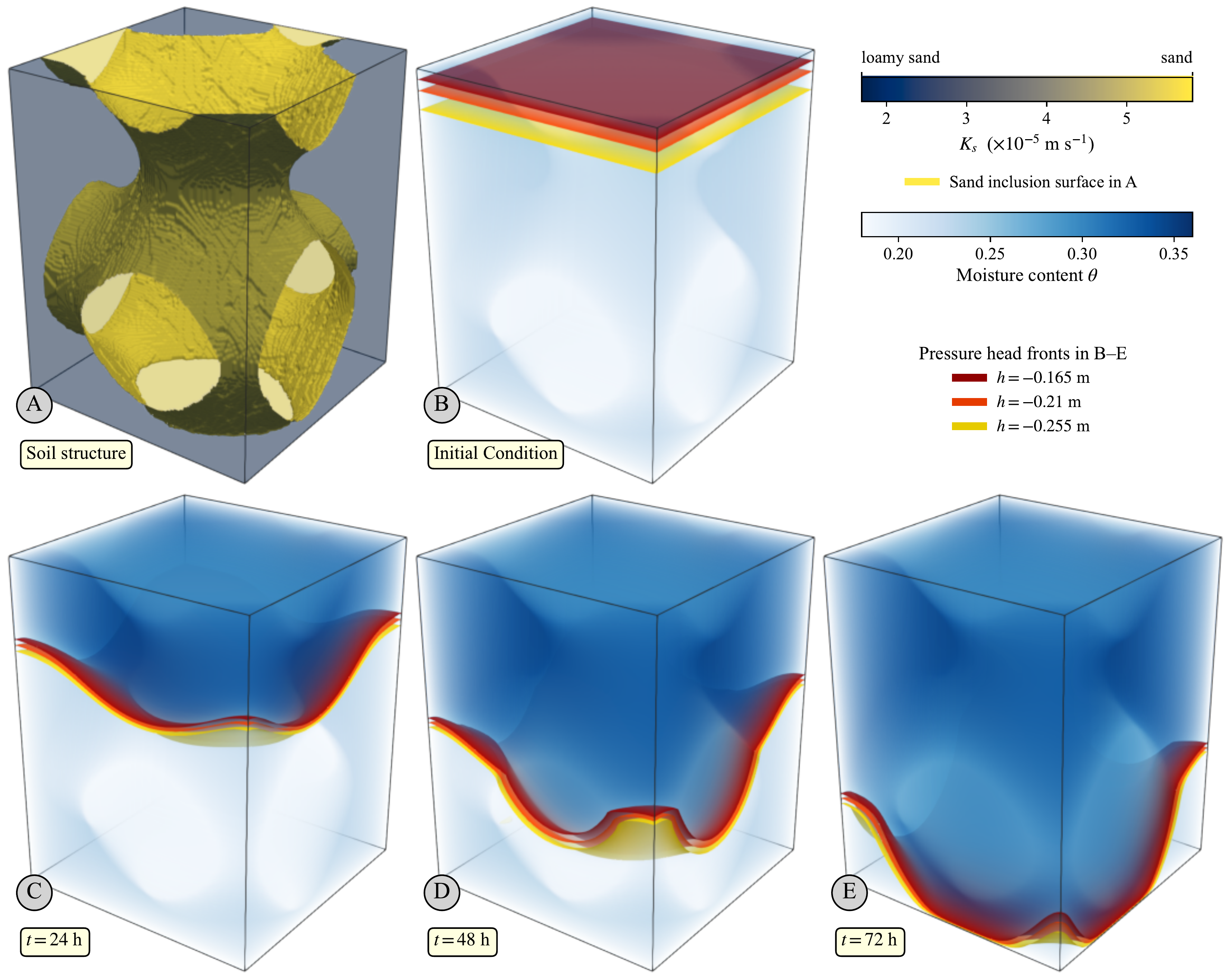
Cockett (2018): 3D infiltration through a heterogeneous conductivity field – reproduces the published SimPEG result.
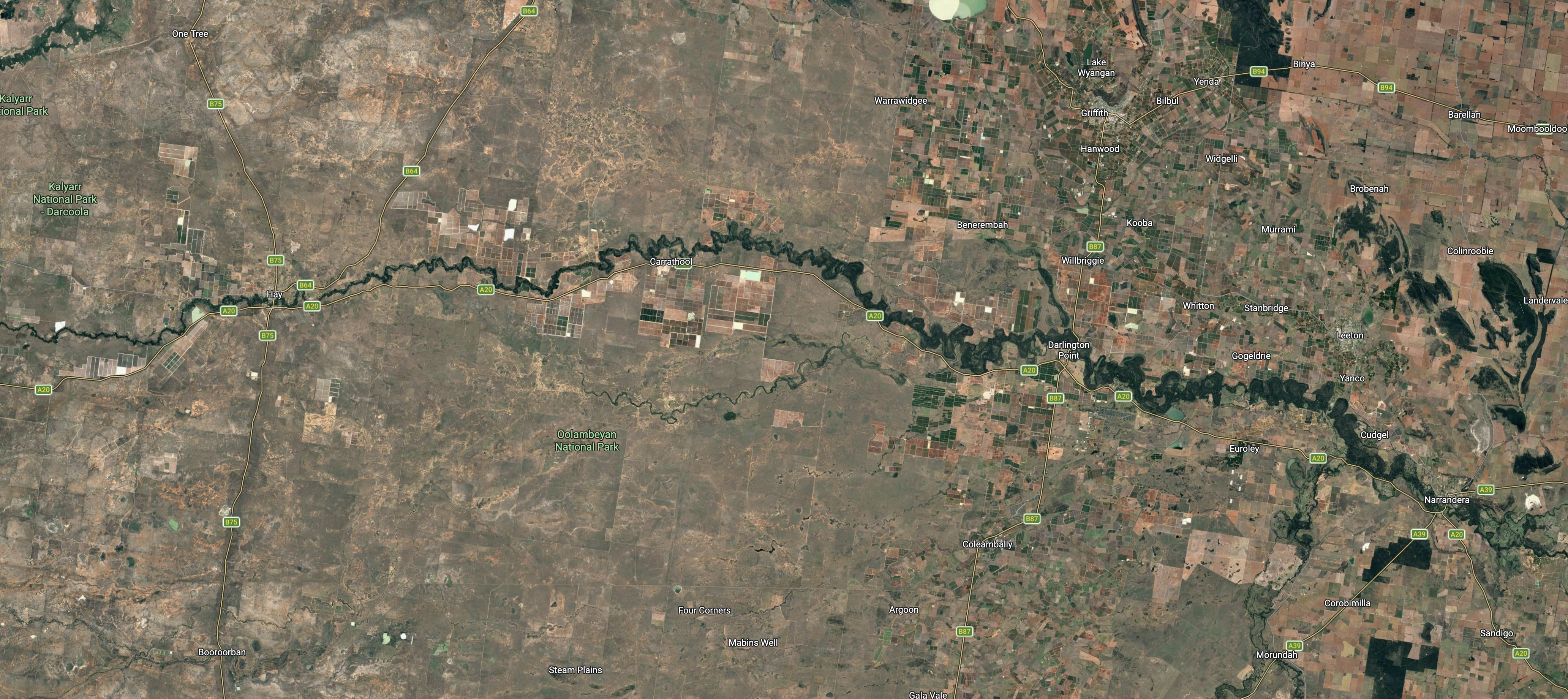
Google Maps
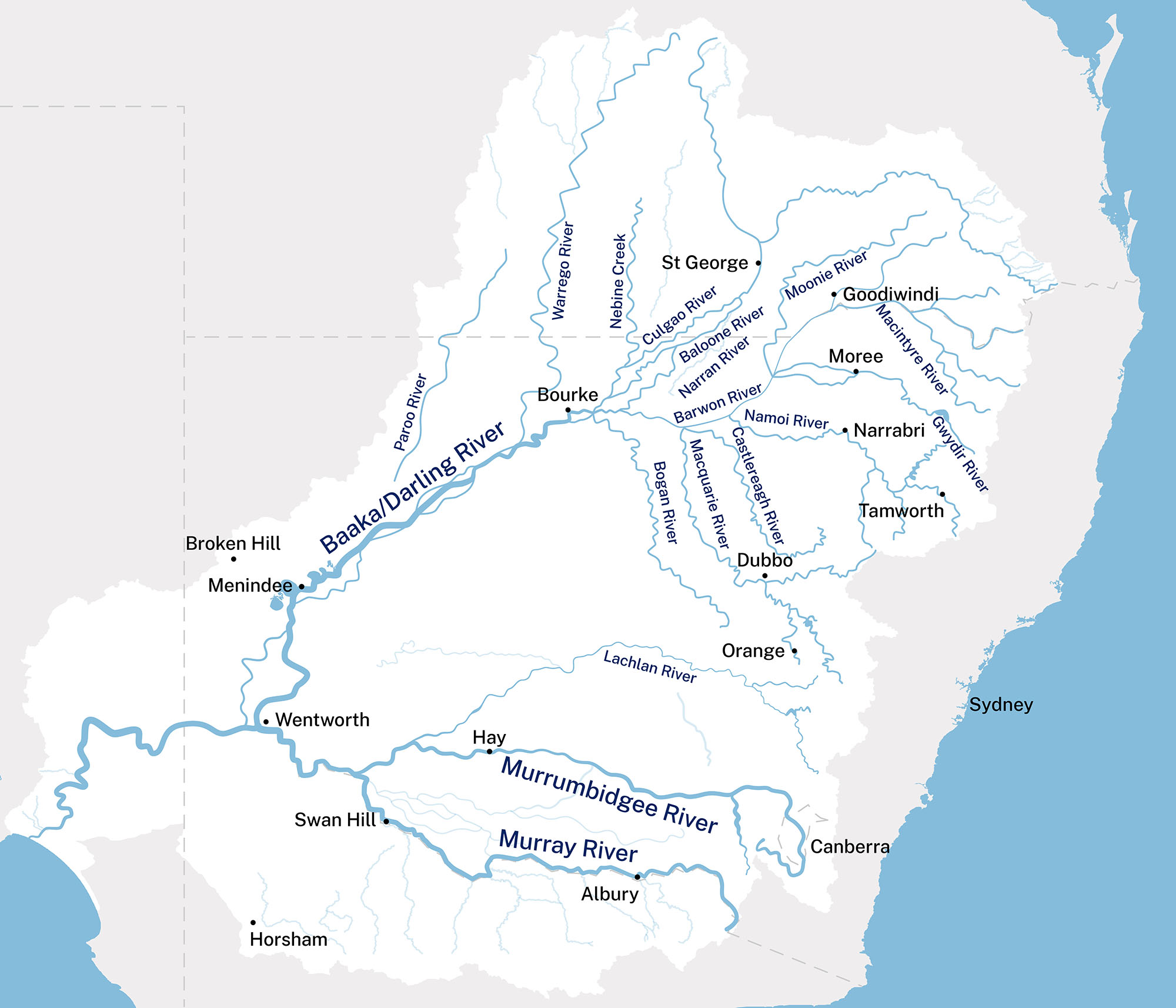
Map of MDB
The target: the Lower Murrumbidgee
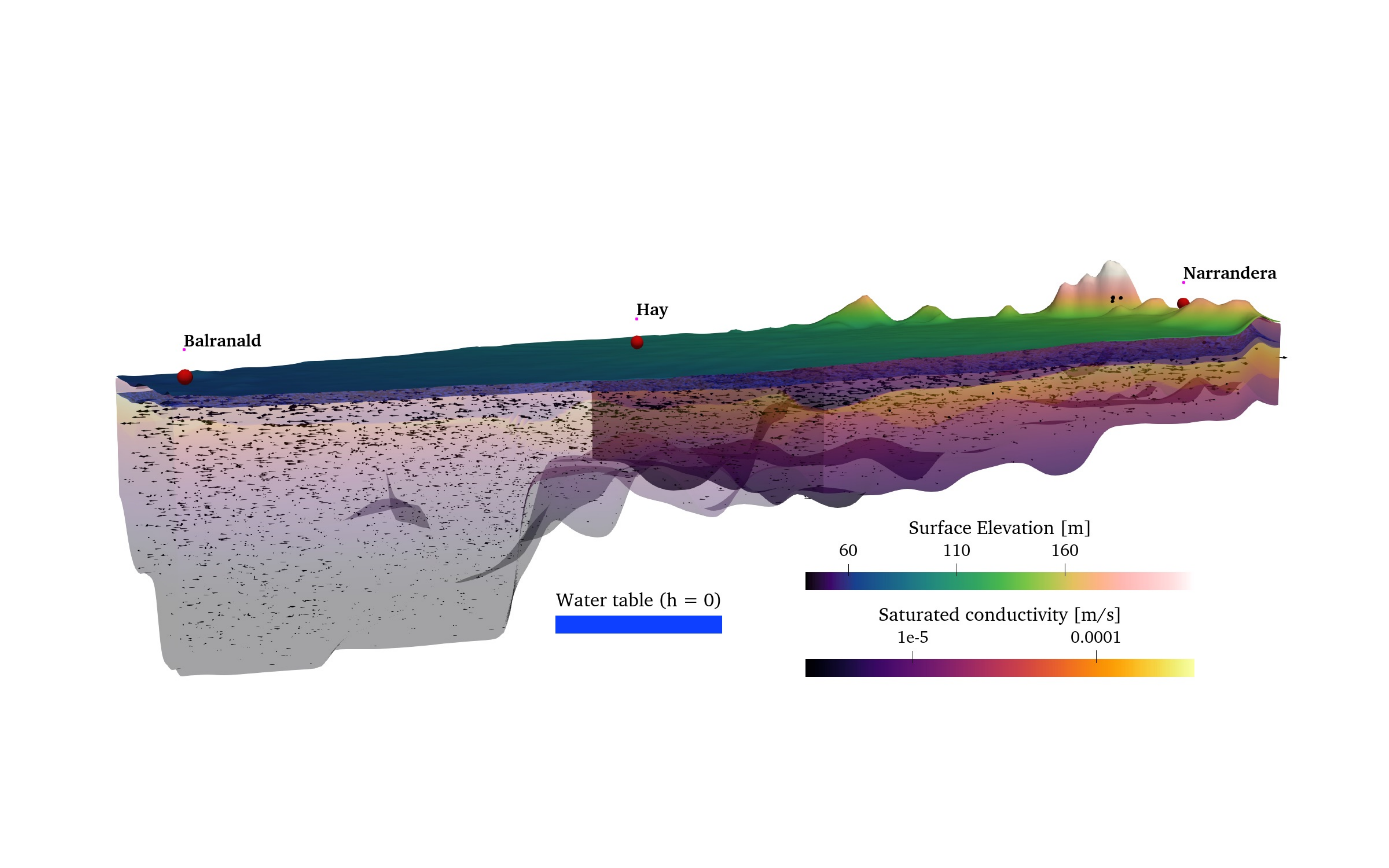
~30,000 km², full 3D variably saturated flow on a terrain-following mesh built from real elevation and borehole data. A demonstration of capability at basin scale – not yet a calibrated forecast.
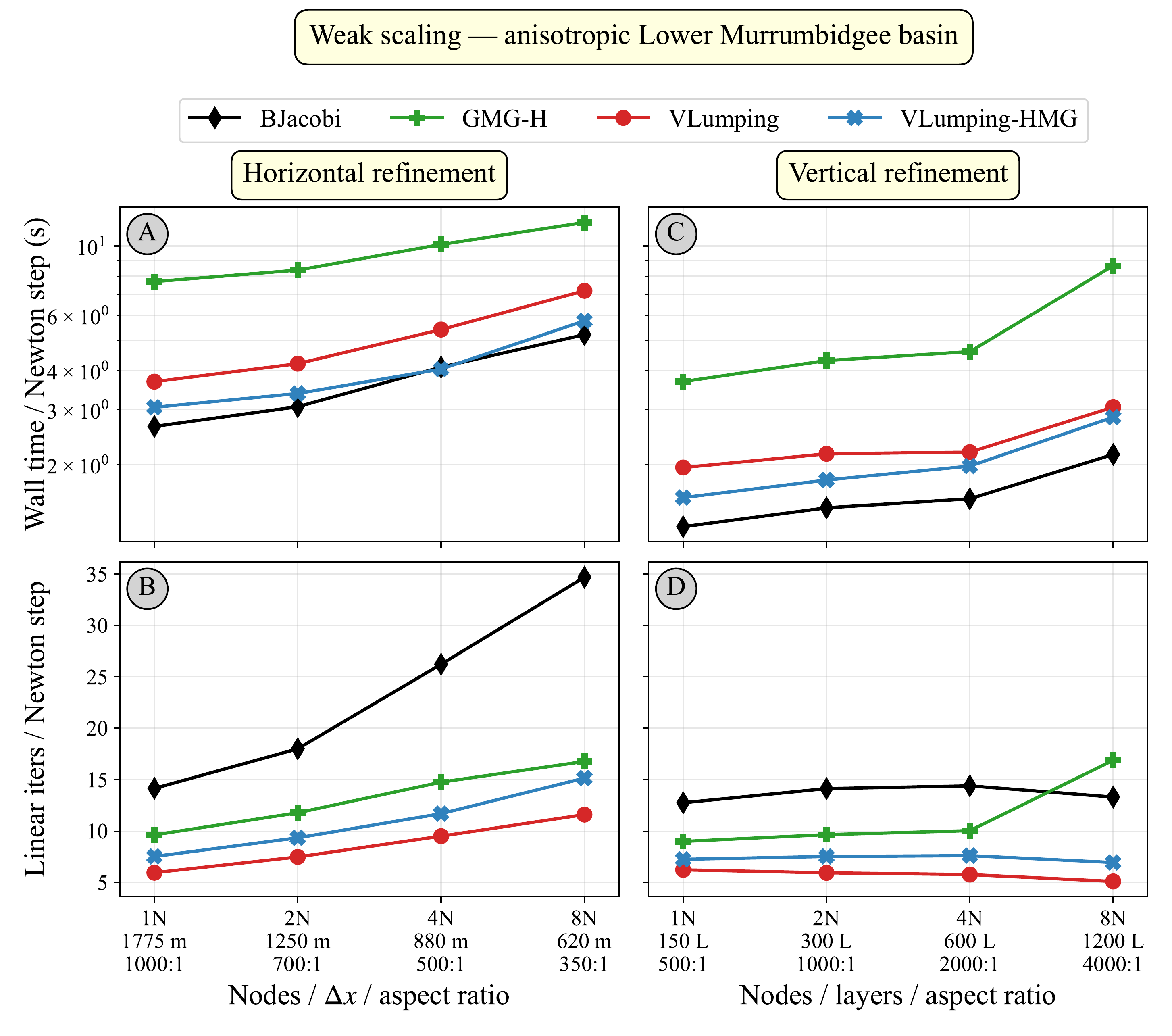
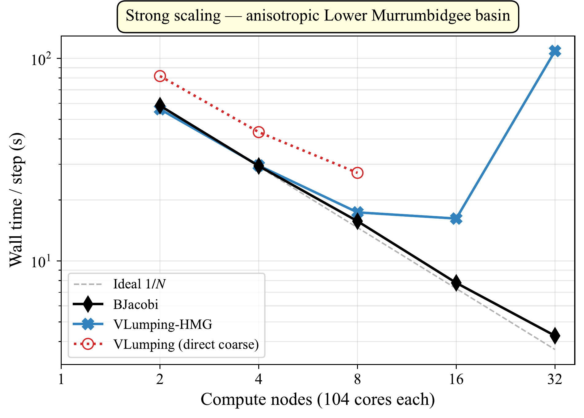
It scales
The point of the preconditioning is that the linear solves stay efficient as the problem grows.
- Weak scaling: hold work per processor fixed, grow the problem – runtime stays flat.
- Strong scaling: fix the problem, add processors – it keeps speeding up.
The vertically lumped preconditioner keeps the iteration count low and flat across the extreme aspect ratios that defeat standard multigrid.
Reliability
Accurate, convergent, mass-conservative.
Scalability
Weak- and strong-scaling at basin scale.
Flexibility
Terrain-following meshes, choice of discretisation.
Connection to data
Real elevation, stratigraphy and borehole data.
Inversion
Adjoint is set up – this is the next piece.
Where this leaves us
We now have a reliable solver for the full Richards’ equation at basin scale.
Forward modelling: done. Inversion and surface coupling: next.